6-reduction
Reduction
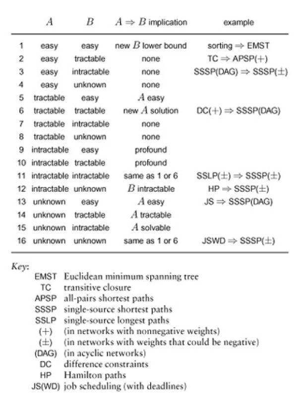
Definition 21.3 We say that a problem A reduces to another problem B if we can use an algorithm that solves B to develop an algorithm that solves A, in a total amount of time that is, in the worst case, no more than a constant times the worst-case running time of the algorithm that solves B. We say that two problems are equivalent if they reduce to each other.
We show that A reduces to B by demonstrating that we can solve any instance of A in three steps.
- Transform it to an instance of B
- Solve that instance of B
- Transform solution of B to be a solution of A
Property 21.12 The transitive-closure problem reduces to the all-pairs shortest-paths problem with nonnegative weights.
Property 21.13 In networks with no constraints on edge weights, the longest-path and shortest-path problems (single-source or all-pairs) are equivalent.
Reduction has 2 primary application in design and analysis of algorithms.
- First, it helps us to classify problems according to their difficulty at an appropriate abstract level without necessarily developing and analyzing full implementations
- We often do reductions to establish lower bounds on the difficulty of solving various problems, to help indicate when to stop looking for better algorithms.
The constraint that the cost of transformations should not dominate is a natural one and often applies.
Job Scheduling Specifically, given a set of jobs (with durations) and a set of precedence constraints, schedule the jobs (find a start time for each) so as to achieve this minimum.
To help us solve this problem we consider the following problem
Difference constraints Assign nonnegative values to a set variables $x_0$ through $x_n $that minimize the value of $x_n$ while satisfying a set of difference constraints on the variables, each of which specifies that the difference between two of the variables must be greater than or equal to a given constant.
Linear Programming Assign nonnegative values to a set of variables $x_0$ through $x_n$ that minimize the value of a specified linear combination of the variables, subject to a set of constraints on the variables, each of which specifies that a given linear combination of the variables must be greater than or equal to a given constant.
Property 21.14 The job-scheduling problem reduces to the difference constraints problem.
Property 21.15 The difference-constraints problem with positive constant is equivalent to single-source longest-path problems in an acyclic network.
Problem 21.8 Job scheduling
#include ”GRAPHbasic.cc“
#include ”GRAPHio.cc“
#include ”LPTdag.cc“
typedef WeightedEdge EDGE;
typedef DenseGRAPH<EDGE> GRAPH;
int main(int argc, char *argv[])
    { 	int i, s, t, N = atoi(argv[1]);
        double duration[N];
        GRAPH G(N, true);
        for (int i = 0; i < N; i++)
        	cin >> duration[i];
        while (cin >> s >> t)
        	G.insert(new EDGE(s, t, duration[s]));
        LPTdag<GRAPH, EDGE> lpt(G);
        for (i = 0; i < N; i++)
        	cout << i << ” “ << lpt.dist(i) << endl;
}
Definition 21.4 A problem instance that admits no solution is said to be infeasible.
Property 21.16 The job-scheduling-with-deadlines problem reduces to the shortest-paths problem (with negative weights allowed).
Read text for insights on lower bounds and upper bounds and NP-hard and feasibility.
Property 21.17 A problem is NP-hard if there is an efficient reduction to it from any NP-hard problem.
Property 21.18 In networks with edge weights that could be negative, shortest-paths problems are NP-hard.
Upper bounds If we have an efficient algorithm for a problem B and can prove that A reduces to B, then we have an efficient algorithm for A. There may exist some other better algorithm for A, but B’s performance is an upper bound on the best that we can do for A.
Lower bounds If we know that any algorithm for problem A has certain resource requirements and we can prove that A reduces to B, then we know that B has at least those same resource requirements, because a better algorithm for B would imply the existence of a better algorithm for A (as long as the cost of the reduction is lower than the cost of B). That is, A’s performance is a lower bound on the best that we can do for B.
Intractability In particular, we can prove a problem to be intractable by showing that an intractable problem reduces to it.