Network Flow
Motivating Problem : Imagine a connected, (integer) weighted, and directed graph as a pipe network where the edges are the pipes and the vertices are splitting points. Each edge has a weight equals to the capacity of the pipe. There are also two special vertices : source s and sink t.
What is the maximum flow (rate) from source s to sink t in this graph ?
Ford Fulkerson’s Method
One solution for max-flow is the ford fulkerson’s method. It is an iterative algorithm that repeatedly finds augmenting path p : A path from s to t that passes through positive weighted edges in the residual path p (bottleneck in this path), ford fulkerson method will do two important steps :
- Decreasing/Increasing the capacity of forward (i to j) / backward(j to i) edges along path by
frespectively. - Ford Fulkerson’s method will repeat this process until there is no more possible augmenting path from source s to sink t anymore which implies that the total flow so far is the maximum flow.
The reason for decreasing the capacity of forward edge is obvious By sendinga flow thru augmenting path p, we will decrease the remaining (residual) capacities of the (forward) edges used in p. The reason for increasing the capacity of backwards edges may not be that obvious, but this step is important for the correctness of Ford Fulkerson’ method.
By increasing the capacity of a backward edge j to i, Ford-Fulkerson method allows future iteration (flow) to cancel (part of) the capcity used by a forward edge (i to j) that was incorrectly used by some flows earlier flow (s).
There are several ways to find an augmenting s-t path in pseudo code above, each with different ways, we show two ways DFS or via BFS.
In DFS run time is $O(|f^|E)$ : where factor $|f^|$ is max flow mf value. There can be cases where augmenting (forward) flow decreases by very small factor.
Edmonds Karp’s Algorithm
A better implementation of Ford Fulkerson’s method is to use BFS for finding the shortest path in terms of number of layers/hops between s and t. Runtime Complexity : $O(n^2)$.
It can be proved after $O(VE)$ iteration of BFS, all augmenting paths will already be exhausted.
int res[MAX_V][MAX_V], mf, f, s, t;		// globals
vi p;				// p stores the BFs spanning tree from s

void augment(int v, int minEdge) { // BFS from s->t
  if(v==s) {f = minEdge; return;} // record minEdge in global f
  else if(p[v] != -1) {
    augment(p[v], min(minEdge,res[p[v]][v]));
    res[[p[v]][v] -= f; res[v][p[v]] += f;
  }
}
        // inside int
mf = 0;
while(1) {
  f = 0;
  // run BFS, compare with original BFS
  vi dist(MAX_V, INF); dist[s] = 0; queue<int> q; q.push(s);
  p.assign(MAX_V,-1); // record BFS tree s->t
  while(!q.empty()) {
    int u = q.front(); q.pop();
    if(u == t) break; // immediately stop BFs if reach sink
    for(int v = 0; v < MAX_V; v++) // this part is slow
      if(res[u][v] > 0 && dist[v] == INF)
        dist[v] = dist[u] + 1, q.push(v), p[v] = u;
  }
}
printf("%d\n",mf);
Note : also see Dicnics-Algorithm for max-flow.
Flow Graph Modeling - Part 1
Using above Edmonds Karp’s code above, solving basic/standard Network Flow problem, especially Max Flow is now simpler.
Its now a matter of
- Recognizing that the problem is indeed a Network Flow problem (requires practice).
- Constructing appropriate flow graph. Initiate the residual matrix
resand set the appropriate values forsandt - Running Edmonds Karp’s code on this flow graph.
Example of Applying and modeling Flow Graph - UVa 259-Software Allocation :
Abridged Problem : given upto 26 apps labeled (‘A’ to ‘Z’), upto 10 computers (numbered 0-9), the number of person who brought in each application that day (one digit positive number [1…9]), list of computers that a particular application can run, and the fact that each computer can run only one application that day. Problem now is to determine whether an allocation (that is, a matching) of application to computer can be done and if so, generate possible allocation. If no, simple print the exclamation mark !
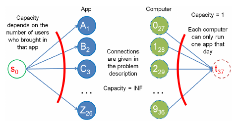
One (bipartite) flow graph formulation is shown, we index vertices from [0…37].
26 + 10 + 2 special = 38.
link source s to all apps and link all computers to sink. All edges are directed. and we set edge weight to number of users bringing that application on that day (capacity) but note 1 computer can process one application so capacity on computer side is set to 1. Edge weight from an app A to a computer is $\infty$.
With this arrangement, if there is a flow from an app A to a computer B and finally to sink t, that flow corresponds to one-matching between that particular app A and computer B.
mf : number of application brought in that day, then we have solution.
Minimum Cut
Let’s define an s-t cut C = (S-component, T-component) as a partition of $V\in G$ s.t. source $s\in S-component$ , $v\in$ T-component. Let’s also define a cut-set of C to be set {$(u,v) \in E | u \in S$ -component, $v \in T$- component } s.t. if all edges in the cut-set of C are removed the Max Flow from s to t is 0. (i.e. s and t are disconnected). The cost of an s-t cut C is defined by the sum of capacities of the edges in the cut-set of C. The minimum cut problem, is to minimize the amount of capacity of an s-t cut. This is more general than finding bridges.
Min Cut has application in sabotaging networks.
Solution is simple : The by-product of computing Max Flow is Min Cut! After max-flow algorithm stops we run graph traversal from source s again. All reachable vertices from source s using positive weighted edges in the residual graph belong to the S-component .All other unreachable vertices belong to T-component. All edges connecting the S-component to T-component belong to the cut-set of C.
(capacity/flow/residual)
Edge 0-3 (30/30/0), edge 2-3 (5/5/0) , edge 2-1 (25/25/0). min cut is 30+5+25 = 60 = max flow value mf. This is minimum over all possible s-t cut
Mult-source/Multi-sink
In case of multiple source and sinks. Create a super source ss and a super sink st. Connect ss with all s with infinite capacity and also connect all t with st with infinite capacity then Edmonds Karp’s as normal.
Vertex Capacities
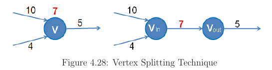
Here a splitting technique shown in case vertex has capacities but sadly it doubles number of vertices in the flow graph. Now with all weights defined on edges, we can run Edmonds Karp’s as normal.
Flow Graph Modeling - Part 2
The hardest part of dealing with Network Flow problem is the modeling of the flow graph. Try to understand the the key steps to derive the required flow graph rather than memorization.
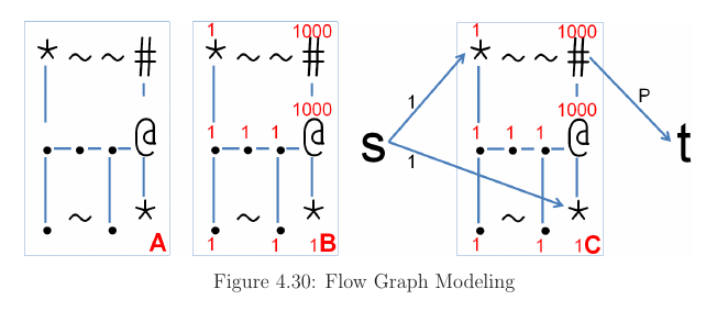
UVa 11380 - you are given a small 2D grid containing these five characters (see Table). You want to put as many ‘*’ (people) as possible to the (various) safe places(s) : the ‘#’ (large wood). The solid and dotted arrows in figure.
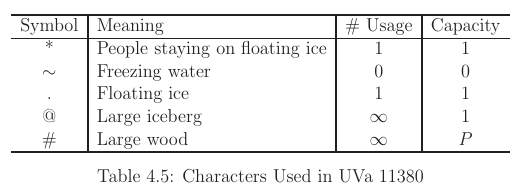
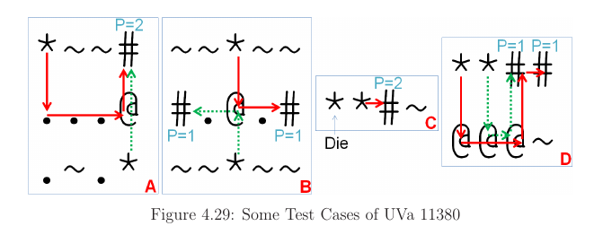
To model the flow graph, we use the following thinking steps. In figure 4.30A, we first connect non ~ cells together with large capacity (1000 is enough). This describes the possible movements in grid. In figure 4.30, we set vertex capacities of ‘*’ and ‘.’ cells to indicate that they can only be used once. Then, we set vertex capacity of ‘@’ and ‘#’ to a large (1000) to indicate that they can be used several times.
In Final figure we create a source vertex s and sink vertex t. Source linked to all ‘*’ with capacity 1 and all ‘#’ are connected to sink with capacity ‘P’ indicateing that large woods can be used P times. Now, the required answer- the number of survivors (s) = equals to the max flow value between s and t of this graph.