7-Breadth First Search
Breadth-First Search
DFS has no relationship to order in which it finds the goal. BFS is based on a shortest path from $v\rightarrow w$ , we start at $v$ and check $w$ among all the vertices that we can reach by following one edge, then we check all the vertices that we can reach by following one edge, then we check all the vertices we can reach by following two edges, and so forth.
When we come to a point where we have to process more than one edges we save them and choose one for current exploration. We use pushdown stack for this purpose.

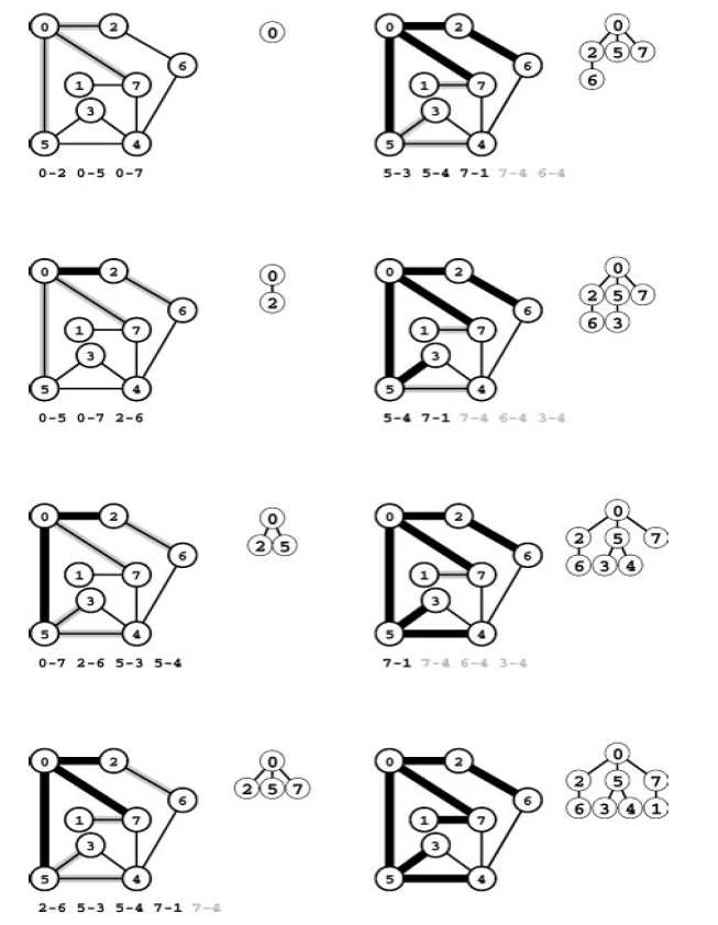
Trace of BFS
Gray edges are used to represent the vertices we can already get to using some other path considered. In BFS we want to explore vertices in order of their distance from start. we can use FIFO queue for this purpose instead of stack.
Strategy
Maintain queue of all edges that connect a visited vertex with an unvisited vertex.
Put a dummy self-loop to start vertex on the queue, then perform the following steps until queue is empty:
- Take edges from the queue until finding one that points to an unvisited vertex.
- Visit that vertex; put onto the queue all the edges that go from that vertex unvisited.
Property 18.9 During BFS, vertices enter and leave the FIFO queue in order of their distance from the start vertex.
Program 18.8 Breadth-first Search
#include <queue>
template <class Graph>
class BFS : public SEARCH<Graph>
{
    vector<int> st;
    void searchC(Edge e){
        queue<edge> Q;
        Q.put(e);
        while(!Q.empty())
            if(ord[(w = Q.get()).v] == -1)
            {
                int v = e.v, w = e.w;
                ord[w] = cnt++; st[w] = v;
                typename Graph::adjIterator A(G,w);
                for(int t = A.beg(); t!= A.end() ; t = A.nxt())
                    if(ord[t] == -1) Q.put(Edge(w,t));
            }
    }
public :
	BFS(Graph &G) : SEARCH<Graph>(G), st(G.V(),-1)
    {search();}
	int ST(int v) const { return st[v];}
};
DFS, we have a forest that characterized the dynamics of the search, one tree for each connected component, one tree node for each graph vertex, and one tree edge for each graph edge.
BFS corresponds to traversing each of the trees in this forest in level order. As with DFS we use a vertex indexed vector.
Program 18.9 Improved BFS
void searchC(Edge e)
{
    queue<Edge> Q;
    Q.put(e); ord[e.w] = cnt++;
    while(!Q.empty())
    {
        e = Q.get(); st[e.w] = e.v;
        typename Graph::adjIterator A(G,e.w);
        for(int t = A.beg(); !A.end(); A.nxt())
            if(ord[t] == -1)
            { Q.put(Edge(e.w,t)); ord[t] = cnt++;}
    }
}
Property 18.10 For any node $w$ in the BFS tree rooted at $v$, the tree path from $v$ to $w$ corresponds to a shortest path from $v \rightarrow w$ in the corresponding graph.
Property 18.11 BFS visits all the vertices and edges in a graph in time proportional to $V^2$ for the adjacency-matrix representation and to $V+E$ for the adjacency-lists representation.
BFS helps in solving the spanning tree, connected components, vertex search and several other basic connectivity problems.
Shortest Path : Find a shortest path in graph from $v$ to $w$. We can accomplish this task by starting a BFS that maintains the parent-link representation st of search tree at $v$, then stopping when we reach $w$. The path up the tree from $w$ to $v$ is shortest path.
after construction a BFS object bfs a client could use this code to print path connecting $w$ to $v$.
for(t = w; t!=v ; t = bfs.ST(t)) cout<<t<<"-";
cout<<v<<endl;
Single-source shortest paths Find shortest paths connecting a given vertex $v$ with each other vertex in the graph. The full BFS tree rooted at $v$ provides a way to accomplish this task : The path from each vertex to the root is a shortest path to the root. Therefore, to solve the problem we run BFS to completion starting at $v$. The st vector that results from this computation is a parent-link representation of BFS tree, and the code in the previous paragraph will give the shortest path to any other vertex $w$.
DFS wends its way through the graph, storing on the stack the points where other parts branch off; BFS sweeps through the graph, using a queue to remember the frontier of visited places.