2-Dijkstras Algorithm
Dijkstra’s Algorithm
In 20.3 we discussed Prim’s algorithm for finding MST of a weighted undirected graph. Here similarly we put source on SPT; then we build the SPT one edge at a time, always taking next the edge that gives a min shortest path from the source to vertex not on the SPT. In other words, we add vertices to SPT in order of their distance to the start vertex. This is known as Dijkstra’s algorithm.
Property 21.2 Dijkstra’s algorithm solves the single-source shortest-paths problem in networks that have nonnegative weights.
We can solve source-sink-shortest-paths problem, if we start at the source and stop when the sink come off the priority queue.
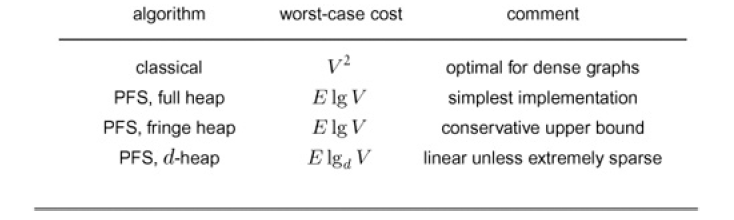
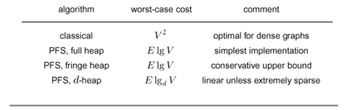
Dijkstra’s original implementation, which is suitable for dense graphs, is precisely like Prim’s MST algorithm. Specifically we simple change the assignment of priority P from p=e->wt() (edge wt) to p=wt[v]+e->wt() ( distance from the source to edge’s destination)
Property 21.3 With Dijkstra’s algorithm, we can find any SPT in a dense network in linear time.
For sparse graphs, we can do better by viewing Dijkstra’s algorithm as a generalized graph-searching method that differs from DFS, from BFS, from Prim’s MST algorithm in only the rule used to add edges to the tree.
This PFS scheme also encompasses Dijkstra’s algorithm. That is, changing the assignment of P in Program 20.7 to p=wt[v]+w->wt() ( the distance from the source to the edge’s destination ) gives an implementation of Dijkstra’s algorithm that is suitable for sparse graphs.
Property 21.4 For all networks and all priority functions, we can compute a spanning tree with PFS in time proportional to the time required for V insert , V delete the minimum , and E decrease key operations in a priority queue of size at most V.
Property 21.5 With a PFS implementation of Dijkstra’s algorithm that uses a heap for the priority-queue implementation, we can compute any SPT in time proportional to E lg V.
Program 21.1 Dijkstra’s algorithm (priority-first search)
template <class Graph, class Edge> class SPT
{
	const Graph &G;
    vector<double> wt;
    vector<Edge *> spt;
    public:
    SPT(const Graph &G, int s): G(G),spt(G.V()),wt(G.V(),G.V())
    {
        PQi<double> pQ(G.V(), wt);
        for(int v = 0; v < G.V(); v++) pQ.insert(v);
        wt[s] = 0.0; pQ.lower(s);
        while(!pQ.empty())
        {int v = pQ.getmin(); // wt[v] = 0.0;
        	if(v!= s && spt[v] == 0 ) return;
         typename Graph::adjIterator A(G,v);
         for(Edge* e= A.beg(); !A.end(); e = A.nxt())
         {
             int w = e->w();
             double P = wt[v] + e->wt();
             if(P<wt[w])
             { wt[w] = P; pQ.lower(w); spt[w] = e; }
         }
        }
    }
    Edge *pathR(int v) const { return spt[v]; }
    double dist(int v) const { return wt[w]; }
};
Property 21.6 Given a graph with V vertices and E edges, let d denote the density E/V. If d < 2, then the running time of Dijkstra’s algorithm is proportional to $V \lg V$. Otherwise, we can improve the worst-case running time by a factor of $\lg(E/V)$, to $O (E \lg_d V )$ (which is linear if E is at least ($V^{1+ε}$)by using a $\lceil E/V \rceil$ -ary heap for the priority queue.
These all four classical graph processing algorithms all can be implemented with PFS, a generalized priority queue based search that build graph spanning tree one edge at a time.
We have also considered four different implementation of PFS. The fist is the classical dense-graph implementation that encompasses Dijkstra’s algorithm and Prim’s MST algorithm (program 20.6) other three are sparse-graph implementation that differ in priority-queue contents :
- fringe edges
- fringe vertices
- all vertices
Cost of implementation of Dijkstra’s algorithm