2 augmeting path maxflow algorithms
Augmenting-Path Maxflow Algorithms
An effective approach to solving maxflow problems was developed by L.R. Ford and D. R. Fulkerson in 1962.
It is a generic method for increasing flow incrementally along paths from source to sink that serves as the basis for family of algorithms. It is know as Ford-Fulkerson methods or augmenting path methods.
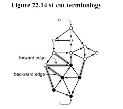
This algorithm will compute the maxflow in some cases, but will fall short in other cases. To improve the algorithm such that it always finds a maxflow consider a more general way to increase flow along any path from source to sink through network’s underlying undirected graph. The edges on any such path are either forward edges, which go with the flow (when we traverse) or backward edges that goes against teh flow.
We can increase the flow in forward edges and decrease in backward edges. The amount by which flow can be increased is limited by min unused capacities in forward edges and the flows in the backward edges.
Summary
Start with zero flow everywhere. Increase the flow along any path from source to sink with no full forward edges or empty backward edges, continuing until there are no such paths in the network.
This method always finds a maxflow, no matter how we choose the paths.
Definition 22.3 An st-cut is a cut that places vertex s in one of its sets and vertex t in the other.
The capacity of an st-cut in a flow network is the sum of capacities of that cut’s st-edges, and the flow across an st-cut is the difference between the sum of the flows in that cut’s st-edges and the sum of the flows in that cut’s t-s edges.
Minimum cut Given an st-network, find an st-cut such that the capacity of no other cut is smaller. For brevity, we refer to such a cut as a mincut, and to the problem of finding one in a network as the mincut problem
Property 22.3 For any st-flow, the flow across each st-cut is equal to the value of the flow.
Property 22.4 No st-flow’s value can exceed the capacity of any st-cut.
Property 22.5 (Maxflow–mincut theorem) The maximum value among all st-flows in a network is equal to the minimum capacity among all st-cuts.
Another implication of the correctness of the Ford–Fulkerson algorithm is that, for any flow network with integer capacities, there exists a maxflow solution where the flows are all integers.
Definition 22.4 Given a flow network and a flow, the residual network for the flow has the same vertices as the original and one or two edges in the residual network for each edge in the original, defined as follows: For each edge v-w in the original, let f be the flow and c the capacity. If f is positive, include an edge w-v in the residual with capacity f ; and if f is less than c, include an edge v-w in the residual with capacity c-f.
Program 22.2 Flow-network edges
class EDGE
{ int pv, pw, pcap, pflow;
public:
    EDGE(int v, int w, int cap) :
        pv(v), pw(w), pcap(cap), pflow(0) { }
    int v() const { return pv; }
    int w() const { return pw; }
    int cap() const { return pcap; }
    int flow() const { return pflow; }
    bool from (int v) const
    	{ return pv == v; }
    int other(int v) const
    	{ return from(v) ? pw : pv; }
    int capRto(int v) const
    	{ return from(v) ? pflow : pcap - pflow; }
    void addflowRto(int v, int d)
    	{ pflow += from(v) ? -d : d; }
};
Program 22.3 Augmenting-paths maxflow implementation
template <class Graph, class Edge> class MAXFLOW
{
  const Graph &G;
    int s,t;
    vector<int> wt;
    vector<Edge *> st;
    int ST(int v) const { return st[v]->other(v); }
    void augment(int s, int t)
    {
        int d = st[t] -> capRto(t);
        for(int v = ST(t); v!= s; v = ST(v))
            if( st[v]->capRto(v) < d)
                d = st[v]->capRto(v);
        st[t]->addflowRto(t,d);
        for(int v = ST(t); v!=s; v = ST(v))
            st[v]->addflowRto(v,d);
    }
    bool pfs();
    public:
    	MAXFLOW(const Graph &G, int s, int t) : G(G),s(s),t(t), st(G.V()), wt(G.V())
        {while(pfs()) augment(s,t);}
};
member functions capRto and addflowRto implement residual network : if e is a pointer to an edge v-w with capacity c and flow f; then e->capRto(w) is c-f and e->capRto(v) is f; e->addflowRto(w,d) adds d to the flow; and e->addflowRto(v,d) subtracts d from the flow
Residual networks allow us to use any generalized graph search to augment path, since any path from source to sink in the residual network corresponds directly to an augmenting path in the original network. Increasing the flow along a path implies making changes in the residual network.
Program 22.4 PFS for augmenting-paths implementation
template <class Graph, class Edge>
bool MAXFLOW<Graph,Edge>::pfs()
{
    PQi(int v = 0; v<G.V(); v++)
    { wt[v] = 0; st[v] = 0; pQ.insert(v);}
	wt[s] = -M; pQ.lower(s);
    while(!pQ.empty())
    {
        int v = pQ.getmin(); wt[v] = -M;
        if(v==t || (v!=s && st[v] == 0)) break;
        typename Graph::adjIterator A(G,v);
        for(Edge* e = A.beg(); !A.end(); e = A.nxt())
        {
            int w = e->other(v);
            int cap = e->capRto(w);
            int P = cap < -wt[v] ? cap : -wt[v];
            if(cap > 0 && -P < wt[w])
            { wt[w] = -P; pQ.lower(w); st[w] = e;}
        }
    }
    return st[t] != 0;
}
A complete analysis establishing which specific method is best is a complex task, however, because their running times depend on
- The number of augmenting paths needed to find a maxflow
- The time needed to find each augmenting path.
These quantities can vary widely, depending on the network being processed and on the graph search strategy.
Simplest Ford-Fulkerson implementation uses shortest augmenting paths. This method was suggested by Edmonds and Karp in 1972.
To implement it, we use a queue for the fringe, either by using the value of an increasing counter for P or by using a queue ADT instead of priority-queue ADT. In this case augmenting path amounts to BFS in residual network. We refer this method as shortest-augmenting-path algorithm
Another one by Edmonds and Karp is : Augment along the path that increases the flow by the largest amount
This we refer as maximum-capacity-augmenting path maxflow algorithm.
Property 22.6 Let M be the maximum edge capacity in the network. The number of augmenting paths needed by any implementation of the Ford– Fulkerson algorithm is at most equal to $VM$.
Such a bound on M can be very large number. Worse it is easy to describe situation where the number of iteration is proportional to maximum edge capacity.
Corollary The time required to find a maxflow is $O(V EM)$, which is $O(V^2M)$ for sparse method.
Property 22.7 The number of augmenting paths needed in the shortest augmenting- path implementation of the Ford–Fulkerson algorithm is at most V E/ 2.
Corollary The time required to find a maxflow in a sparse network is $O (V^3)$.
Worst case performance may not be useful for predicting performance in a practical application.
Property 22.8 The number of augmenting paths needed in the maximal augmenting- path implementation of the Ford–Fulkerson algorithm is at most $2E \lg M$.
Corollary The time required to find a maxflow in a sparse network is $O (V^2 \lg M \lg V )$.
Maxflow Algorithm with better worst case bounds have been discovered, and no nontrivial lower bound has been proved that is possibility of linear-time algorithm remains.
One direct improvement is using value of decreasing P or a stack implementation for the generalized queue. The intuition is that method is fast and easy to implement, and appears to put flow throughout the network. As we will see it varies according to the graphs we run it on.
Another alternative is to use randomized-queue implementation for the generalized queue so that search for augmenting path is randomized search. This method is fast and easy to implement;. It may embody the good features of DFS and BFS. Randomization is a powerful tool in algorithm design, and this problem represent a reasonable situation in which to consider using it.
We conclude this section by looking more closely at methods that we have examined in order to see the difficulty of comparing them or attempting the performance for practical applications.
Perhaps the most important lesson that we can learn from studying particular networks in detail in this way is that the gap between the upper bounds of Properties 22.6 through 22.8 and the actual number of augmenting paths that the algorithms need for a given application might be enormous. For example, the flow network illustrated in Program 22.23 has 177 vertices and 2000 edges of capacity less than 100, so the value of the quantity $2E \lg M$ in Property 22.8 is more than 25,000; but the maximum capacity algorithm finds the maxflow with only seven augmenting paths. Similarly, the value of the quantity $V E/2$ in Property 22.7 for this network is 177,000, but the shortest-path algorithm needs only 37 paths.